I want to use HT-ATES in my simulation
Tested for version 22.7.0-g778faf5-main of the ESDL MapEditor and version 0.4.6 of Computational Framework (CF)
This tutorial focus on how to use High Temperature Aquifer Thermal Energy Storage (HT-ATES) in the simulation. HT-ATES is simulated using TNO in-house tool called ROSIM and Doubletcalc3D. For more information regarding this model please visit this link
This tutorial shows the steps to find the answer to the following questions:
How to add HT-ATES in the MapEditor?
How to use HT-ATES and heatpump in the MapEditor?
How to set properties and run simulation in CF?
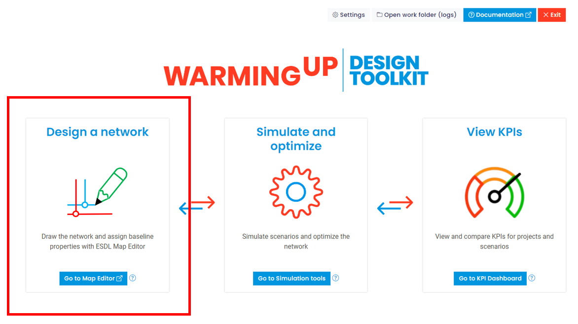
To achieve these results the following workflows and packages are used:
|
ESDL MapEditor is used to create a network. |
|
The network is loaded into the Computational Framework (CF), which allows to alter heat demand, simulate and optimize heat networks, define (sub) scenario’s and related modifiers. |
|
In the CF environment, CHESS is used to simulate the network. |


1 |
How to add HT-ATES in the MapEditor? |
|---|---|
1.1 |
Go to the MapEditor and use credentials to login.
|
1.2 |
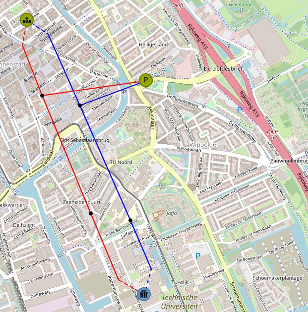
Create a simple network consist of 2 producers (1 for base load and 1 for peak load) and 1 demand.
|
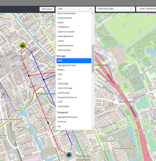
1.3 |
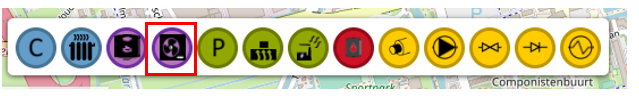
Add HT-ATES asset in to the MapEditor by selecting from Asset Dropdown List. |
1.4 |
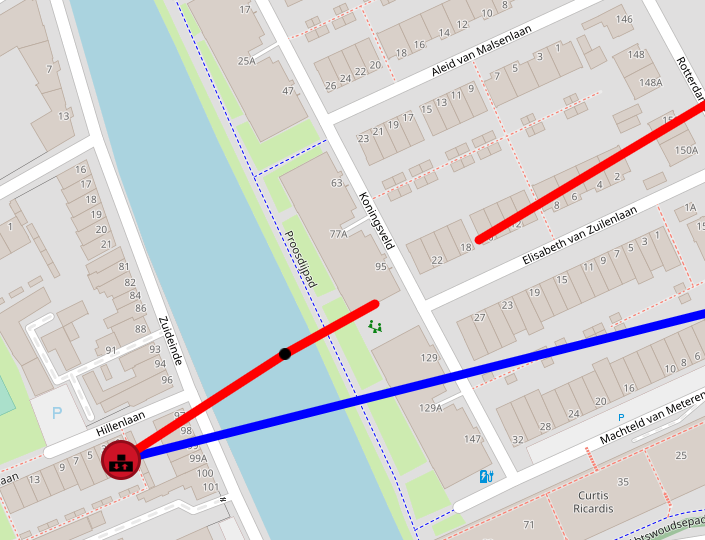
Connect supply pipe to the InPort of ATES and return pipe to the OutPort of ATES (Similar to connecting a Heat Demand). |
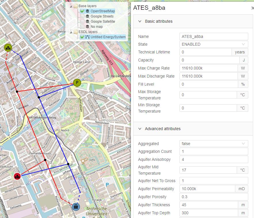
1.5 |
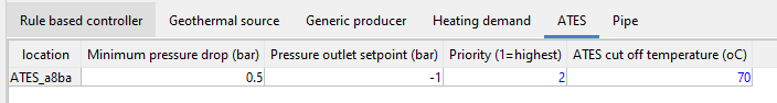
Fill ATES properties:
|
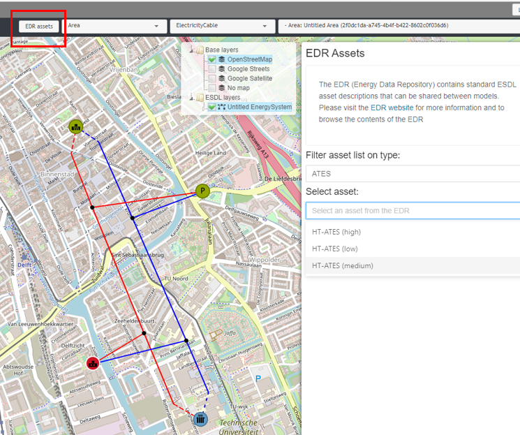
1.6 |
If you don’t have subsurface information/knowledge, you can select a HT-ATES system from the Energy Data Repository (EDR). There are 3 default HT-ATES with either low, medium or high performance based on poor, medium or good subsurface conditions. Without any subsurface knowledge the ‘medium’ option is advised. The user can compare results: ‘what impact does lower or higher quality of subsurface conditions for a HT-ATES system have on my results?’ by running all three options.
|
2 |
How to use HT-ATES and heatpump in the MapEditor? |
|---|---|
2.1 |
ATES hot well temperature will drop during production period. It is not desirable when you are connecting it directly to the primary grid. Thus, you can add a heat pump when the temperature drops below the grid temperature.
|
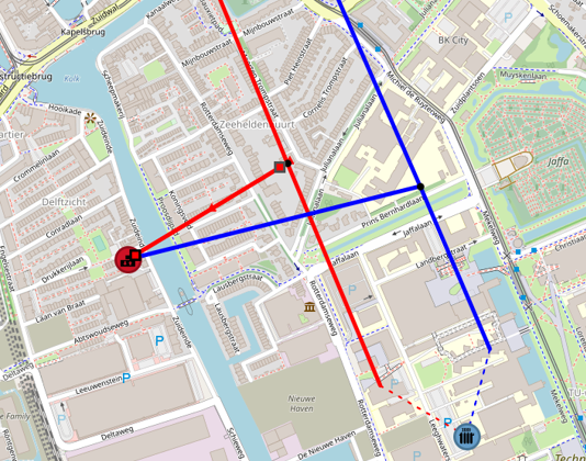
2.2 |
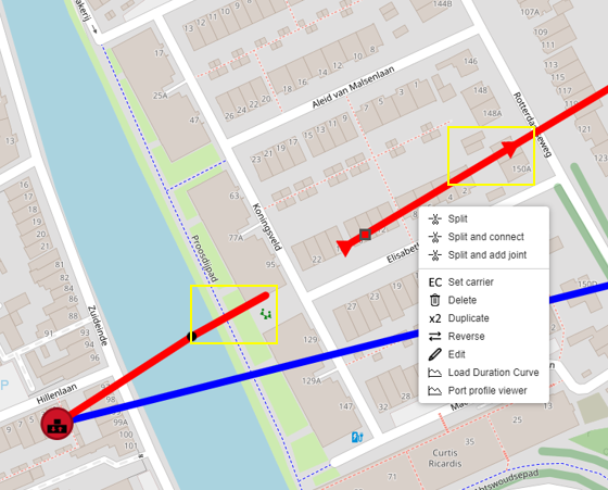
Split the supply pipe into 3 segments (1 of them with a Joint, and 1 of them just Split, not connected):
|
2.3 |
Right click and select Reverse for pipes with yellow box. Make sure the supply pipe connected to ATES is still having direction going to the ATES.
|
2.4 |
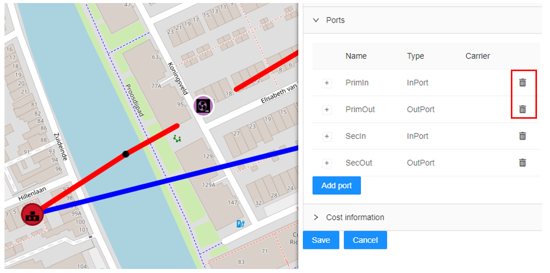
Add Heat Pump and remove (PrimIn Port and PrimOut Port)
|
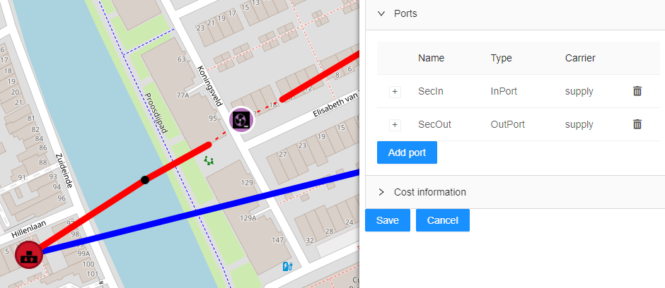
2.5 |
Connect the SecIn and SecOut port of the heat pump to the pipes.
|
2.6 |
Note: With this 2 ports heat pump, we are upgrading heat from ATES to meet the grid’s temperature from Secondary side. At the moment, the 4 ports heat pump is not supported for ATES because ATES flow is bidirectional for charging and discharging. The 4 ports heat pump is only for 1 direction flow like a producer (e.g. geothermal). Thus, during discharging, we can’t have lower temperature than your return pipe’s temperature for injection to the cold well. |
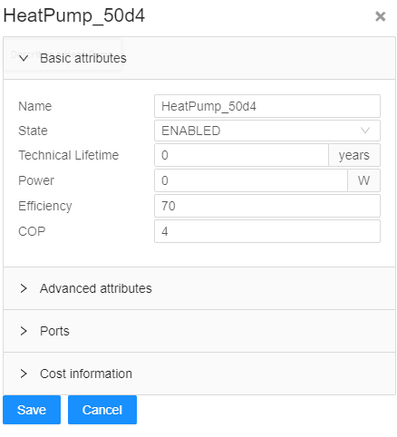
2.7 |
Fill the heat pump’s properties:
|
3 |
How to set properties and run simulation in CF? |
3.1 |
Go to the Simulate and optimize and create a new project. Open CF.
|
3.2 |
Import and set Demand Profiles
|
3.3 |
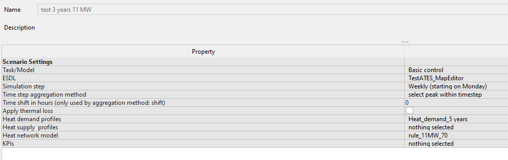
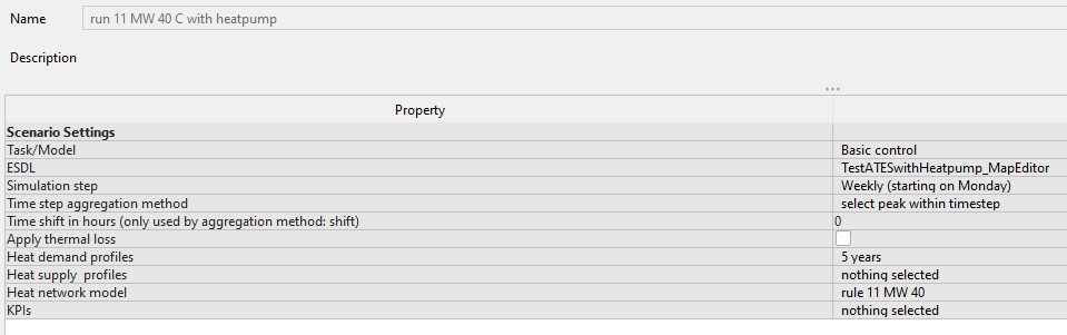
Set simulation settings:
|
3.4 |
Run simulation for 3.5 years with weekly timesteps and peak demand.
|
3.5 |
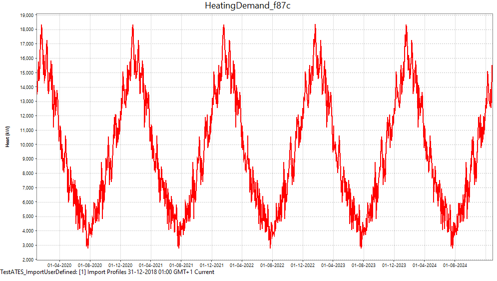
Check the results when simulation is finish.
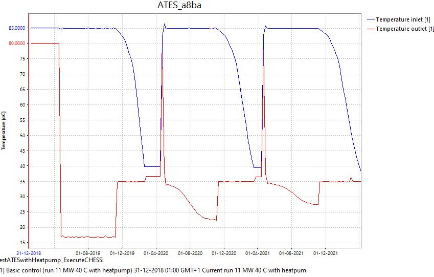
As we can see from figure above that ATES is used to cover the peak load and stops supplying the heat when temperature drops below 70 C. Then, the boiler is taking over the peak load. |
3.6 |
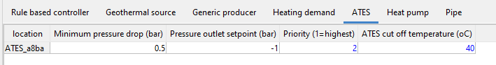
Now, we open the project for ATES with a heat pump. We redo all the settings, but now we reduce the cut off temperature to 40 C. So the ATES will produce longer.
|
3.7 |
Set the heat pump properties such a way it represents the configuration of 4 ports heat pump:
|
3.8 |
Run simulation for 3.5 years with weekly timesteps and peak demand.
|
3.9 |
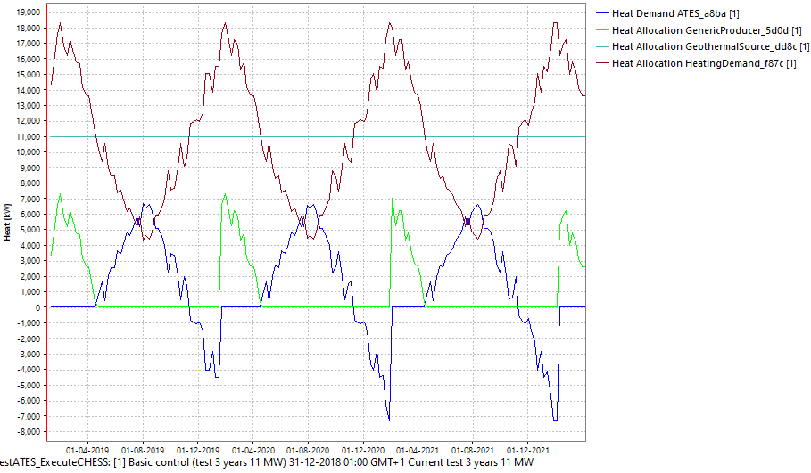
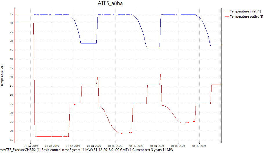
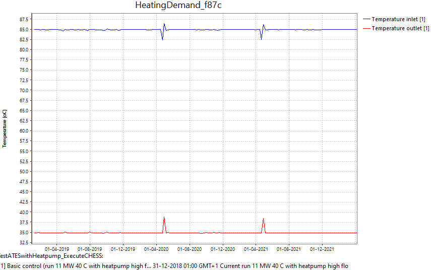
Check the results when simulation is finish.
Since the cut off temperature of the ATES can be lower to 40 C, it has a longer operational time during discharge period. So the use of the boiler is decreasing over the year. The inlet temperature at Demand remains at grid’s supply temperature of 85 C |