I want to simulate my network with market-based control
Tested for version 22.4.2-g0abbaa1-main of the ESDL MapEditor.
This tutorial focusses on using HeatMatcher to utilize market-based control in a network. Be advised that this is an advanced option in the WarmingUp toolkit and requires some extra skills on using ESDL and configuring it correctly for HeatMatcher market-based control in the toolkit.
Short introduction on HeatMatcher
When you simulate a network in the WarmingUp toolkit, you can specify the order of the dispatch of the different heat supply options for the CHESS network simulator. For some operational scenarios this does not always match practice, as the dispatch of some supply options are dependent on prices that fluctuate throughout the year. Market-based control with HeatMatcher can help in these situations, as it allows you to define the eagerness to supply based on external data such as price information.
In HeatMatcher all assets become part of a virtual market, where they can bid on energy: what price are they willing to pay or receive for a certain amount of energy. The bidding strategy is implemented in agents that represent each asset, hence the name of agent-based control. When all agents have placed their bid, HeatMatcher determines where demand matches supply and calculates the market clearing price. This price is used in each agent to determine how much energy the assets have to consume or produce in the next time step. The function that calculates the bid is dependent on the role in the market (e.g. producer, consumer, storage), the type of asset and business strategy and is in this setup provided by HeatMatcher. These bid functions can be extended for more sophisticated bidding behaviour (out of the scope of this tutorial). In the current HeatMatcher, it allows you to specify the marginal cost of the bid. The marginal cost of an asset is the price at which producing becomes profitable and consuming becomes not profitable. If used as a static value, it provides similar behaviour as setting the priority of the asset’s dispatch, but HeatMatcher also supports marginal cost profiles as input, for example marginal costs based on the electricity market price, allowing for dynamic marginal costs in a simulation.
Note: In the beta release of the WarmingUp toolkit, all prices are normalized. This means that the maximum market price is set a 1 and all prices need to be defined between 0 and 1 (i.e. divided by the maximum price in the market).
Tutorial Outline
This tutorial shows the steps to simulate a simple network using market-based control.
As this is an advanced tutorial, it is assumed that the other tutorials on using the ESDL mapeditor and the Computational framework are already known.
This tutorial shows the steps to find the answer to the following questions:
How to create an ESDL that describes the required input for market-based control?
How to simulate a market-based control scenario?
To achieve these results the following workflows and packages are used:
|
ESDL MapEditor is used to create a network and configure market-based control. |
|
The network is loaded into the computational framework (CF), which allows us to configure the simulation, run the simulation and view the results. |


1 |
How to create an ESDL that describes the required input for market-based control? |
1.1 |
Load the desired network into the ESDL mapeditor. |
1.2 |
For each producer and consumer asset, configure the marginal costs. This can be done in two ways:
|
1.2.1 |
Specify static marginal costs |
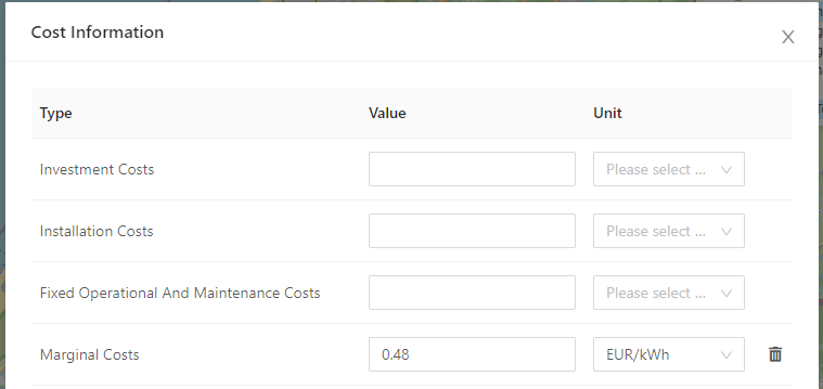
Open the properties of the asset by clicking on it and expand the Cost Information widget. Click the “Change or add cost” button and specify the marginal cost field in the window that pops up.
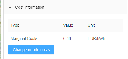
Use a value between 0 and 1 (due to normalisation as described in the introduction). Also select a unit (e.g. EUR/kWh, is not used in the simulation) When closing the popup window, the sidebar looks similar to the screenshot below.
|
|
1.2.2 |
Specify dynamic marginal costs (advanced) |
1.2.2.1 |
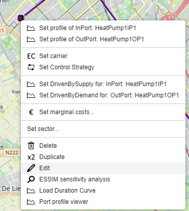
This advanced scenario describes how you can add a profile instead of a single value to the marginal costs of an assets, as currently the MapEditor GUI does not allow to directly edit these marginal costs. For HeatMatcher we need to add a Cost profile to the cost information of the asset, and specify the marginal costs there. As ESDL supports multiple profile types (e.g. manual specified, from a database, etc) for this tutorial we use an InfluxDBProfile as we assume that the profile data is present in the database by uploading an CSV file using the profile upload tool in the ESDL MapEditor (see View->Settings, Profiles plugin). Make sure that the profile contains hourly data (or better) and is in range of your simulation period (currently 01-01-2019 – 01-01-2020. Alternatively, you can use a TimeSeries profile where each value needs to be filled in manually if the simulation only concerns a short timespan (e.g. 24 hours). Right-click on the assets and select ‘Edit’, to open up the ESDL Browser, which shows the semantic definition of the asset.
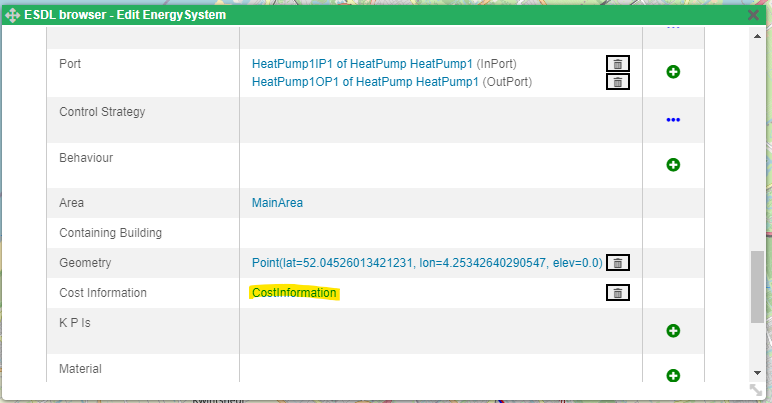
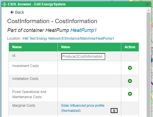
Scroll down to the CostInformation section of this asset (in the example a HeatPump) and select the InPort of the asset.
After clicking on the CostInformation the following dialog appears (if there is no CostInformation link to click on, press the (+) button in the last column of the Cost Information row if the link is not present.
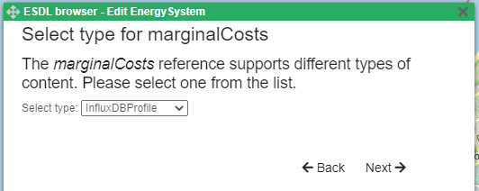
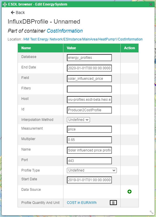
Select InfluxDBProfile from the drop down list and press ‘Next’. Copy the information of the profile that you’ve previously uploaded using the Profile plugin in the Settings dialog (under View->Settings, Profile plugin).
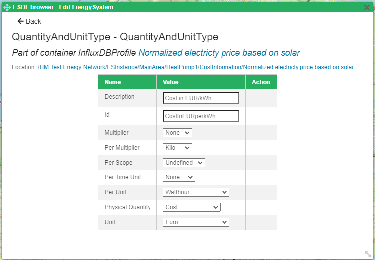
Furthermore it is important to specify the “Profile Quantity and Unit” in the last row of the dialog.
Make sure you specify ‘Cost’ as physical quantity.
|
1.2.2.2 |
Save the network to the ESDL drive using File -> Save to ESDL Drive … |
2 |
Simulate the network in the Computational Framework (CF) |
Open the toolkit and select Simulate and optimize. Import the network design from the ESDL Drive that was created in the previous scenario. Press the ‘Simulate and optimize’ button to load the network in CF (this might take a few seconds). |
|
2.1 |
Import profiles |
In the CF task window select ‘Import Profiles’ and press the play button ( |
|
2.2 |
Configure Market-based control |
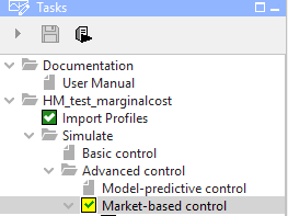
In the task window, navigate to Simulate -> Advanced control and then Market-based control.
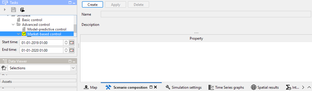
And subsequently select “Scenario composition” to configure the scenario for Martket-based control. This window allows you to create a new scenario and specify the timestep.
This will an empty view
|
|
2.3 |
Configure timestep |
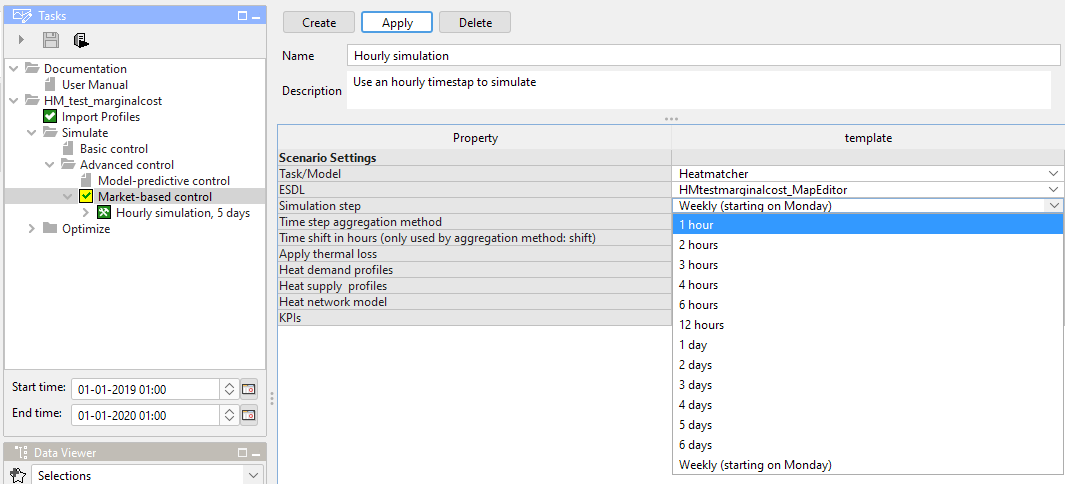
The default timestep in CF is 1 week, but when using price profiles a smaller timestep is needed. Select ‘1 hour’ from the drop down list and give the scenario a name.
Press ‘Apply’ to use this configuration of the simulation. |
|
2.4 |
Configure simulation time range |
By default CF simulates a full year. When stepping by a 1 hour timestep, this simulation will take considerable amount of time. Therefore select a time range below the Tasks window that fits your requirements. |
|
2.5 |
Simulate |
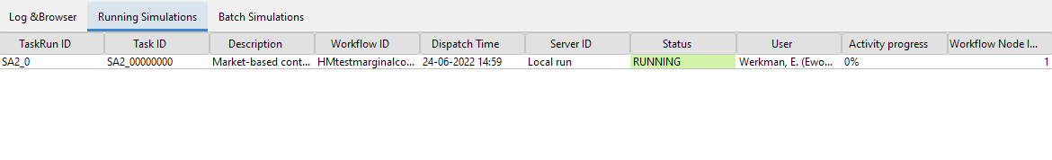
Select the newly created scenario in the Tasks window and press the play button to simulate this scenario. In the Logging windows (select the Logging tab on the bottom right) you can see the progress of the running simulation (select ‘Running simulation’ at the top).
|
|
2.6 |
Explore results |
Explore the results of the simulation in the graphs section of CF. |